What are Mean, Median, Mode and Range?
If you examine the world around you, you’ll find that data is everywhere. Weather reports, sports statistics, and your grades in school: these are just a few examples of data that you might encounter in your day-to-day life. It’s easy to be overwhelmed by the sheer quantity of data, especially with modern technology making more and more data available to us every day.
Thankfully, mathematics gives us tools to help us summarize large sets of data with just a few numbers. In this blog, we’ll cover the mean, median, mode, and range, which are four different numbers that you can use to help you understand the datasets you encounter in school and in your own life.
Before we talk about these four specific statistics, let’s talk about two important categories of statistics that can help us understand different aspects of datasets. These two categories are measures of central tendency and measures of dispersion.
A measure of central tendency is used to approximate the center of a dataset (think central → center). The mean, median, and mode are examples of measures of central tendency. A measure of dispersion is used to approximate how spread out a dataset is (think dispersion → dispersed/spread out).
The range is an example of a measure of dispersion. By using measures of central tendency and measures of dispersion, we can get an idea of both the middle of the dataset as well as its extremities. While they don’t give us the full picture, measures of central tendency and dispersion are valuable information when doing data analysis.
To get a better understanding of the mean, median, mode, and range, it helps to work with an example data set. Let’s imagine you survey everyone in your class and ask each person how many times they’ve watched a certain movie. The data you get could look something like this:
0, 1, 1, 0, 1, 0, 8, 2, 2, 2, 4, 2, 1, 3, 2, 1, 3, 2, 1, 6, 1, 0, 1, 4, 1, 3.
It is hard to extract much information when the data is presented as just a list of numbers, so let’s visualize the data using a bar graph.
The height of each bar in this graph represents the number of times a student watched the movie. Looking at this graph, you might notice that most students watched the movie two or fewer times, but there are a few students who watched the movie more than twice. Something you might want to know is how many movies the “typical” student watched. To answer that question, we’ll use measures of central tendency.
What is the Mean?
The first measure of central tendency we’ll discuss is the mean, which is also known as the average. We can interpret the mean as the result of “sharing” all of the data equally across the dataset. Let’s go into more detail about what that means.
If you wanted to share something equally with your friends, you might first find out how much of that thing you all have in total, and then you could split up that total so that you and your friends all get the same amount. We can follow a similar two-step process to compute the mean of our dataset.
First, we want to find out how many times the movie was watched by the class in total. To do this, we add up how many times each student watched the movie to get the total for the whole class.
0+1+1+0+1+0+8+2+2+2+4+2+1+3+2+1+3+2+1+6+1+0+1+4+1+3 = 52
Now that we have the total number of times the movie was watched in the class, we can go on to the next step, which is to divide this total by the number of students surveyed in the class. Remember that when we do a division problem like 12 / 4, we are answering the question “If I split 12 evenly into 4 groups, how much is in each group?”
This is exactly the type of problem we are trying to solve when sharing something equally, so division is the correct operation for the job. If you count the number of entries we have in our dataset, you’ll find that there are 26. Now, dividing the total number of times the movie was watched, 52, by the number of students surveyed, will give us the value of the mean:
Mean = 52 / 26 = 2.
Our calculations show that when we share the total number of movie-watchings equally with all of the students in the class, each student would have watched the movie 2 times. Therefore, we can say that the mean of our dataset is 2.
We can extend the process we followed for this specific dataset into a formula that will work for all datasets. Here is the formula to calculate the mean of any dataset:
Mean = (x1 + x2 + … + xn) /n
In this formula, we are considering a dataset with n elements. In our example, n would be equal to 26 since that is the number of students that were surveyed. x1 represents the first entry in the dataset, x2 represents the second entry, and so on, until we reach xn, the last entry in the dataset.
This is an important formula to remember, but if you are having a hard time memorizing it or understanding it, try to remember the two-step process we followed to calculate the mean: first add all of the entries in the dataset to get a total, and then divide that total by the number of entries in the dataset. If you remember this, you’ll be able to calculate the mean of any dataset you encounter.
To get a more visual understanding of what the mean is telling us, take a look at the below two graphs. In the first graph, all of the students who watched the movie more than twice have the upper parts of their bars colored red.
This represents how many more times they watched the movie compared to the mean value. In the second graph, we redistribute this red excess to the students who watched fewer than two times. Because the mean of this dataset is 2, when we finish redistributing the excess, all of the bars have a height of exactly 2.
What is the Median?
The median is another measure of central tendency. The median splits a dataset into two halves. The lower half contains values less than or equal to the median, and the upper half contains values that are greater than or equal to the median.
If you know the median of a dataset, then you know that about 50% of the values in the dataset are below the median and about 50% of the values are above the median. To find the median, it is a good idea to sort your dataset because this will make it easier to determine how to split it in half. Here is what we get when we sort our dataset:
0, 0, 0, 0, 1, 1, 1, 1, 1, 1, 1, 1, 1, 2, 2, 2, 2, 2, 2, 3, 3, 3, 4, 4, 6, 8.
Now, because our dataset has 26 values in it, when we split the dataset in half, each half should have 13 values. Since we’ve sorted our dataset, that means that the first 13 values in the dataset will make up the lower half of the dataset and the last 13 values in the dataset will make up the upper half.
Lower Half | 0, 0, 0, 0, 1, 1, 1, 1, 1, 1, 1, 1, 1, || 2, 2, 2, 2, 2, 2, 3, 3, 3, 4, 4, 6, 8 | UpperHalf
You’ll notice that we don’t have any values in between the lower and upper halves of the dataset. This is because 26 is an even number, so when we divide it into two halves, we don’t have anything left over. To get the median in this case, we take the two values that are closest to the middle and then calculate the number that is halfway between those two values.
To calculate this halfway number (which is also known as the midpoint), we add the two numbers together and then divide by 2. For this dataset, the values that are closest to the middle are 1 and 2, so the median is 1.5 since (1+2)/2 = 1.5. If we had an odd number of values, then we would have an extra value in the middle which would be the median of the dataset.
We can understand the median visually by adding a horizontal line to the bar graph of our dataset at the height of the median. Since the median of our dataset is 1.5, we can draw a horizontal line 1.5 units above the bottom of the graph.
When we draw this line, we can count the number of bars that are below the median line and the number of bars that go above the median line, and we’ll find that 13 bars are below the line and the other 13 bars are above the line.
This is exactly what we expect since we know the median splits our dataset into a lower half and an upper half. If your dataset has elements that are equal to the median, then you might not get a perfect 50-50 split, but the median splits typical datasets into two roughly equal halves.

In some datasets, the median can be a more reliable measure of central tendency than the mean because it is less sensitive to extreme values. To explain what this means, let’s recall how we calculated the mean.
To find the mean, we added up all of the numbers in our dataset, and then divided by the number of points in our dataset. Meanwhile, to calculate the median, we first sorted the dataset, but only used the number(s) that were in the middle.
This means that if a dataset contains outliers, or values that are much higher or much lower than the bulk of the values in the dataset, the mean will be influenced by those outliers because they are included in the first addition step, but the median will be less influenced by those outliers because the median only cares about the values in the middle.
Depending on what you are trying to study, one measure of central tendency might be better than another, so it is good to know how to calculate both the mean and the median.
What is the Mode?
The mode is the last measure of central tendency we’ll discuss in this post. The mode is the value that occurs the most often in a dataset. To calculate the mode for a dataset, you count how many times each value occurs in the dataset, and choose the value or values that have the highest number of occurrences.
One way to keep track of how many times each value occurs is with a frequency table. A frequency table has two columns. The first column is a list of all of the unique values in the dataset and the second column is the frequency of that value, or how many times it occurred in the dataset.
In between these two columns, it can be helpful to include a tally column for you to track each value as it appears in the dataset and then count up all of the tally marks for each row and put the result in the frequency column. Here is what the frequency table for our dataset would look like:
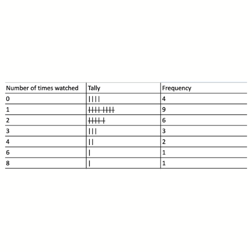
From this frequency table, we can see that 1 is the value that occurs the most often with a frequency of 9, so that is the mode for our dataset.
One of the unique aspects of the mode is that it can be applied to qualitative data. So far we have only been talking about quantitative data, which is data that can be represented with numbers. However, we can also analyze qualitative data, which is data that is not measured with numbers.
An example of a qualitative dataset would be survey responses on what your classmates’ favorite foods are. The elements of this dataset could include things like “pasta” or “ice cream”. As opposed to how many times someone watched a movie, a person’s favorite food can’t be represented with just a number. You can’t add, subtract, multiply, or divide things in this dataset, and you can’t put them in order from least to greatest, which means that there is no way to calculate a mean or median.
However, we could create a frequency table for this favorite foods dataset and use that to find the mode, which would be the food that is selected as the favorite by most students.
What is the Range?
Unlike the three other statistics we’ve discussed so far, the range is a measure of dispersion, not a measure of central tendency. The range tells you how “wide” your dataset is. A dataset with a large range has values that are spread out over a larger interval, whereas a dataset with a small range has values that are confined to a smaller interval.
If your data is sorted, then the range is easy to find. The range is equal to the largest entry in the dataset minus the smallest entry in the dataset. The largest value in a dataset is called the maximum, and the smallest value in the dataset is called in the minimum. Therefore, we can write the formula for the range as
Range = Maximum - Minimum.
In our example dataset, the maximum is 8 and the minimum is 0, so the range is equal to 8-0, or 8. In a bar graph of a dataset, the range can be seen visually as the height difference between the tallest bar (maximum) and the lowest bar (minimum). You can see this visual representation of the range in the graph below. Notice that since the minimum of this dataset is 0, the lowest bar can’t be seen on the graph, so we just measure to the bottom of the graph.
—
The range can be a useful statistic because it gives you an idea of the variability in your data. If there is a lot of variation in your data (some values are very high and some values are very low), this will be reflected by your range being larger.
On the other hand, if your dataset has less variation and all of the values are in the same ballpark, then this will be reflected by your range being smaller. However, you should be aware that if your data has an outlier, or a value that is either much higher or much lower than the bulk of your dataset, then the range could mislead you into thinking your data is very spread out even if the dataset is otherwise relatively close together.
Sample Problem
Now it is your turn to calculate the mean, median, mode, and range of a dataset. Try doing all of your calculations before looking at the solution so you can learn from your mistakes.
The following dataset represents the ages of 13 randomly selected students in your school.
13, 18, 17, 16, 17, 15, 18, 14, 14, 14, 15, 17, 13
Mean
Mean = (13+18+17+16+17+15+18+14+14+14+15+17+13)/13 = 201/13 ≈ 15.5
Notice that the mean of this dataset is a decimal number that is not in the original dataset. This is a common occurrence, so don’t worry if you get a number that is not in the original dataset when calculating the mean.
Median
Median
|
v
Lower Half -> |13 13 14 14 14 15| 15 |16 17 17 17 18 18| <- Upper Half
To find the median, we first sort the dataset and then try to split it in half. Since this dataset has 13 elements, each half should contain 6 elements because 13/2=6.5. We can’t have half of an element, so the most we can put in each half is 6. Because the dataset in this example has an odd number of elements, the dataset doesn’t split evenly into halves and we have one element left over. This leftover element is the median.
Mode
Here is the frequency table of this dataset:

From this table we can see that there are two values with a frequency of 3: 14 and 17. Because 14 and 17 have the highest frequency out of all of the values in the dataset, we say that 14 and 17 are the modes of this dataset. A dataset with more than one mode is called multimodal. In our case, because this dataset has exactly two modes, we can call this dataset bimodal.
Range
Range = Maximum - Minimum = 18 - 13 = 5
The largest number that appears in the dataset is 18, so that is the maximum, and the smallest number that appears in the dataset is 13, so that is the minimum.
Final Thoughts on Mean, Median, Mode, and Range
Now you have some tools that you can use to analyze data. However, this is just the start of what you can do with statistics. If you need support in this topic, or others, you can always sign up for a free tutoring session with an UPchieve tutor who can help you get the understanding you need to succeed!